Linear Rational Spline Flows

In this blog post, I am going to summarize our work on linear rational spline flows, which was published at the 23rd International Conference on Artificial Intelligence and Statistics (AISTATS). I will first provide a brief overview of normalizing flows and coupling layer transformations that are a popular approach to construct such models. Then, I will briefly go over our approach to designing coupling layer transformations for flow-based modeling. Note that this is only a very brief introduction to normalizing flows. For a thorough review, see these awesome surveys [Papamakarios et al., Kobyzev et al.].

Normalizing Flows: what are they?!

Imagine that we have a dataset, and we wish to generate more samples of this dataset. To this end, normalizing flows attempt to consider the data as i.i.d samples of an unknown probability density. Parameters of this probability distribution are then adjusted so that they match the samples of the given dataset. Normalizing flows use the change of variables formula to formulate such a distribution. So, if we want to give a one-sentence summary of normalizing flows we can say that they are a flexible family of probability distributions that allow us to fit any data observations to a density function. In this sense, they are just like other methods of density estimation such as kernel density estimation.

To understand the change of variables formula, let’s assume that we have a bunch of i.i.d random vector observations \(\mathbf{x}_1\), \(\mathbf{x}_2\), \(\dots\), \(\mathbf{x}_n\), where \(\mathbf{x}_i \in \mathbb{R}^d\). Flow-based models assume that there is a certain density behind the generation of such samples. To model this density, let \(\mathbf{Z}~\sim~p(\mathbf{z})\) denote a random vector with a well-known distribution such as standard normal. This density is referred to as the base distribution. Now, to re-shape this universal base density into our data distribution, we pass \(\mathbf{Z}\) through a transformation \(\mathbf{f}_{\boldsymbol{\theta}}(\cdot)\) to construct what we believe is our data \(\mathbf{X}=\mathbf{f}_{\boldsymbol{\theta}}(\mathbf{Z})\). Here, \({\boldsymbol{\theta}}\) is the set of parameters that we aim to optimize to fit our parametric model to the data distribution. In flow-based modeling, we are looking to write down the data distribution \(p_\boldsymbol{\theta}(\mathbf{x})\) explicitly. Hence, this transformation \(\mathbf{f}_{\boldsymbol{\theta}}(\cdot)\) has to satisfy certain properties so that we can make use of the change of variables formula. Specifically, if we assume that \(\mathbf{f}_{\boldsymbol{\theta}}(\cdot)\) is invertible and differentiable, then the change of variables formula allows us to connect the base distribution \(p(\mathbf{z})\) to our data density \(p_\boldsymbol{\theta}(\mathbf{x})\) by:

The multiplicative term on the right-hand side is known as the absolute value of the Jacobian determinant. This term accounts for the change in the volume of \(\mathbf{Z}\) due to applying \(\mathbf{f}_{\boldsymbol{\theta}}(\cdot)\). A challenge in designing practical flow-based models is to deal with the computational complexity of this term. As you know, computing determinant of a general \(d \times d\) matrix requires \(\mathcal{O}(d^3)\) operations which is burdensome. In the next section, we will introduce coupling layer transformations that by design reduce this computational cost to \(\mathcal{O}(d)\) operations.

Now that we have defined our density function by an invertible and differentiable transformation, we can use maximum likelihood estimation to find the set of parameters \({\boldsymbol{\theta}}\):

Note that a nice property of the change of variables formula is that it allows for a straightforward composition of multiple flow-based models. To understand this property, let’s assume that instead of trying to map \(\mathbf{Z}\) to \(\mathbf{X}\) using a single transformation, we break down \(\mathbf{f}_{\boldsymbol{\theta}}(\cdot)\) as a composition of \(K\) number of invertible and differentiable transformations:

This transformation is shown in the following figure.

Using the chain rule and the fact that \(\mathrm{det}(AB) = \mathrm{det}(A)~\mathrm{det}(B)\), we can write the log-likelihood of our overall transformation as:

Now that we understood the principles of normalizing flows, it is time to see how we can construct an invertible and differentiable transformation using neural networks.

Coupling Layer Transformations

In the previous section, we saw that normalizing flows need an invertible, differentiable transformation. Also, we need to reduce the computational complexity of the Jacobian determinant to have a practical transformation. Note that since we can compose different flow-based models easily, we may choose a simple transformation for each \(\mathbf{f}_{k}\) and then compose many of them together to build a very expressive transformation. In this sense, they are like ordinary neural networks: instead of trying to come up with a complex shallow network, we choose to have a simple deep one.

A popular approach to building such transformations is through coupling layers [Dinh et al.]. In a single coupling layer, we split the data into two equal parts. We send half of the data to the next layer without changing it. The other half, however, is send through an invertible, differentiable transformation that is parametrized based on the first half of the data. This special structure results in a lower-triangular Jacobian. Thus, computing the Jacobian determinant is going to cost \(\mathcal{O}(d)\).

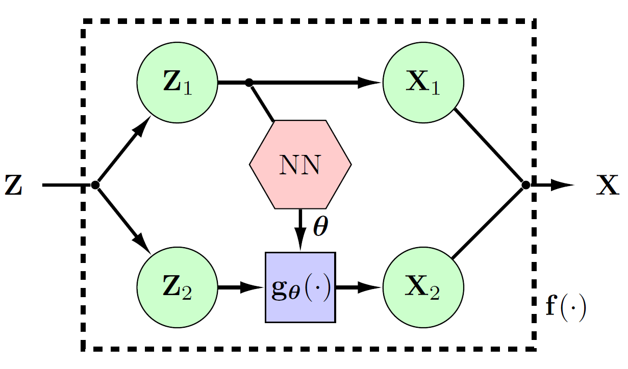
In particular, let’s assume again that we have some data \(\mathbf{z} \in \mathbb{R}^{d}\) that we want to transform using \(\mathbf{f}(\cdot)\). In a coupling layer, we first split the data into two parts \(\mathbf{z}_1, \mathbf{z}_2 \in \mathbb{R}^{d/2}\). Based on this splitting, we transform the data using:

In this equation, \(\mathbf{g}_{\pmb{\theta}({\mathbf{x}_1})}(\cdot)\) is an invertible, differentiable, and element-wise transformation with parameters \(\pmb{\theta}({\mathbf{x}_1})\). As you can see, our parameters \(\pmb{\theta}\) are computed using the first half of the data \({\mathbf{x}_1}\). As such, the Jacobian of this type of transformation is always lower-triangular. The inverse of this transformation can also be computed via

As seen, the inverse of the overall transformation does not depend on the parameter function \(\pmb{\theta}(\cdot)\) to be invertible. Thus, we can use any general function as our parameter function \(\pmb{\theta}(\cdot)\). In the literature, neural networks and their variants (such as CNNs, ResNets, etc.) are usually used.

Below you can see a figure of a single coupling layer.

Now, one may ask that this way, half of the data does not go under any transformation! To deal with this problem, we change the role of \(\mathbf{z}_1\) and \(\mathbf{z}_2\) parts in consecutive layers. In other words, if in the current layer, we keep \(\mathbf{z}_1\) fixed and transform \(\mathbf{z}_2\), in the next layer, we fix \(\mathbf{z}_2\) and transform \(\mathbf{z}_1\).

Although this type of transformation seems simplistic, it can model very complicated data such as images with thousands of pixels. Of course, the more expressive our \(\mathbf{g}\), the more powerful our overall transformation. However, we have to be careful as using complex transformations may require a lot of computational power. For more information about coupling layers, see the surveys introduced in the beginning.

Linear Rational Splines for Flow-based Modeling

Now that we introduced normalizing flows and coupling layers, it is time to see how we can construct one using linear rational splines. We saw that in Eq. (1) we need an invertible, differentiable, and element-wise transformation \(\mathbf{g}(\cdot)\). We also said that this transformation is defined through a set of parameters \(\pmb{\theta}(\cdot)\) that are determined using a function of arbitrary complexity.

In this work, we propose to formulate each element of the mapping \(\mathbf{g}(\cdot)\) using linear rational splines (LRS). In particular, LRS’s are piece-wise functions where each of the pieces are linear rational functions of the form \(y=\tfrac{ax+b}{cx+d}\). Two key elements of an LRS are its number of intervals (bins) and their locations. In the context of spline functions, each bin boundary points are called knots.

LRS’s are not invertible in general. Hence, we need to find a workaround to make them invertible. On the bright side, LRS’s are differentiable inside each interval. The only concern is at the knot points, which need to be \(\mathcal{C}^1\) continuous. Fuhr & Kallay propose an algorithm to construct such monotone (and as a result, invertible) and continuous LRS’s.

Consider this alternative problem: let’s say that we have the knot locations \(\big\{\big(x^{(k)},~y^{(k)}\big)\big\}_{k=0}^{K}\), and assume that they are monotone, meaning that for all \(x_i < x_j\) we have \(y_i < y_j\). Also, let’s assume to know the derivatives at these locations \({\big\{d^{(k)}>0\big\}_{k=0}^{K}}\). Now, we want to fit a monotone, differentiable LRS to such knot points.

To solve this problem, we should evaluate the value and also the derivative of the knot points. Then, we should make sure that these values are equal to each other. Consider the interval \(\big[x^{(k)}, x^{(k+1)}\big]\), where \(x^{(k)}\) and \(x^{(k+1)}\) are two consecutive knot points. Let \(g(x)\) denote our linear rational function for. We can re-write this function as

where \(0~<~\phi=\big(x-x^{(k)}\big)/\big(x^{(k+1)}-x^{(k)}\big)~<~1\). Moreover, \(w^{(k)}\) and \(w^{(k+1)}\) are two arbitrary weights. Using this re-parameterization, we see that \(g(x^{(k)})=y^{(k)}\) and \(g(x^{(k+1)})=y^{(k+1)}\) are automatically satisfied. As seen, we are only left with one degree of freedom (the ratio of w^{(k+1)} to w^{(k)}). However, we still need two degrees of freedom to satisfy the derivative constraints at the start and end of the interval. What should we do?

Fuhr & Kallay resolve this issue by adding an intermediate knot point. In particular, they assume that we have an intermediate point \(x^{(m)} = (1-\lambda) x^{(k)} + \lambda x^{(k+1)}\), where \(0<\lambda<1\). Instead of trying to fit a single LRS to the interval \(\big[x^{(k)}, x^{(k+1)}\big]\), Fuhr & Kallay suggest to fit two of them to the intervals \(\big[x^{(k)}, x^{(m)}\big]\) and \(\big[x^{(m)}, x^{(k+1)}\big]\). The value and also derivative of the intermediate point \(x^{(m)}\) are then treated as free parameters, providing us with the required degree of freedom to satisfy the derivative constraint. Assume that for each interval \(\big[x^{(k)}, x^{(k+1)}\big]\), we assign an intermediate point using \(\lambda^{(k)}\). Fuhr & Kallay show that we can find monotone, \(\mathcal{C}^1\) continuous LRS of the form:

for appropriate set of parameters \(w^{(k)}\), \(w^{(m)}\), \(w^{(k+1)}\). The complete algorithm can be found in our paper. Below, you can see a monotone and differentiable LRS interpolation for six arbitrary knots using different values of \(\lambda\).

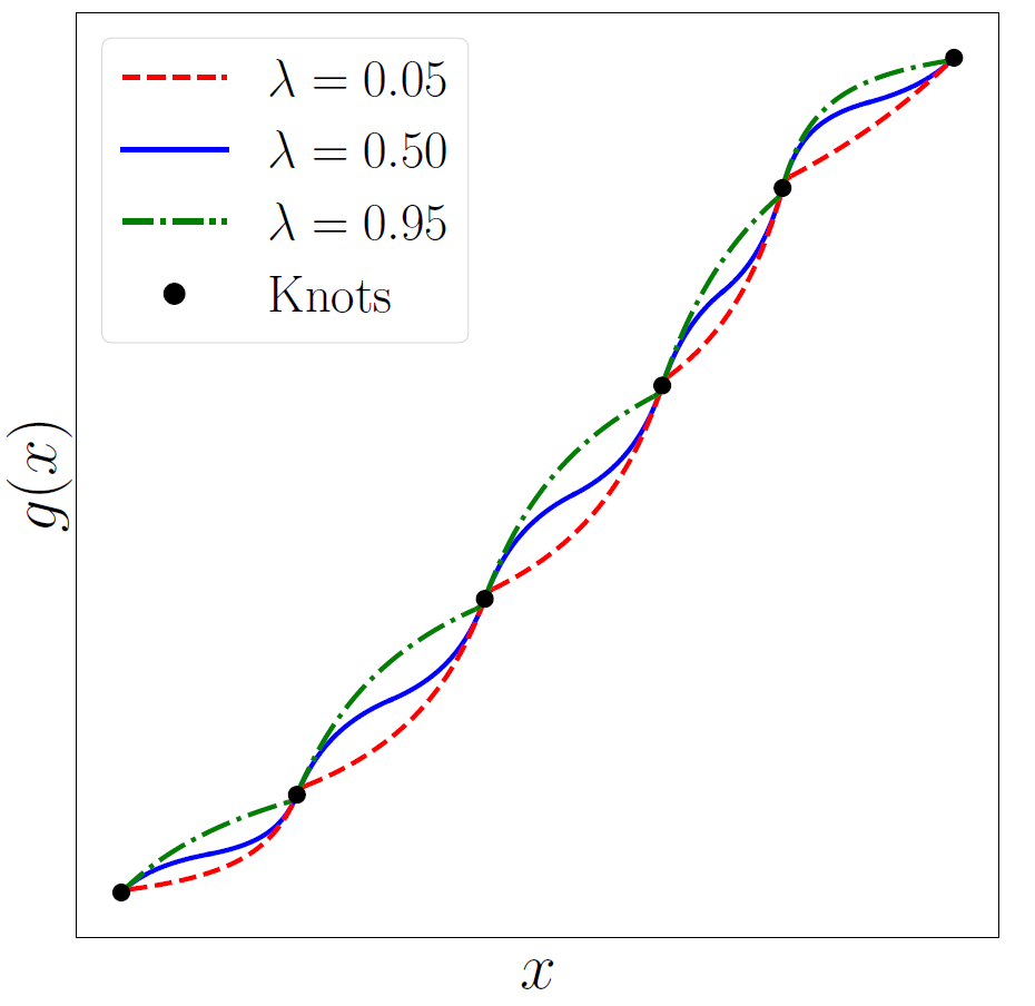
One may ask: what does all this have to do with a flow-based model? Remember that for a coupling layer, we needed an invertible, element-wise, and differentiable function \(\mathbf{g}(\cdot)\). Our idea is to use LRS’s as \(\mathbf{g}(\cdot)\). To this end, we need to specify the number of knot points, their location, and also the first derivative. We consider all of these as our parameter set \(\pmb{\theta}\). As stated in the previous section, these parameters are the output of a function \(\pmb{\theta}(\cdot)\) that takes the fixed half of the data as input. We then use the algorithm of Fuhr & Kallay for monotone LRS fitting to specify our function \(\mathbf{g}(\cdot)\). And ta-da, we finally have a normalizing flow! :D

Simulation Results: Synthetic 2d Data

As a simple example, we showcase the ability of our framework in estimating a synthetic 2d data distribution. Let’s assume that we have the following data samples, and we want to find its underlying probability distribution.

We construct a two-layer flow-based model, where we use coupling layers with LRS transformations. We then use stochastic gradient descent to maximize the log-likelihood objective. Here, we use a uniform distribution as our base density. The following image shows the estimated probability density. It is awesome, isn’t it? ;)

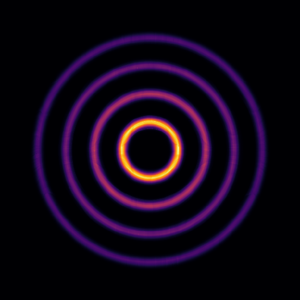
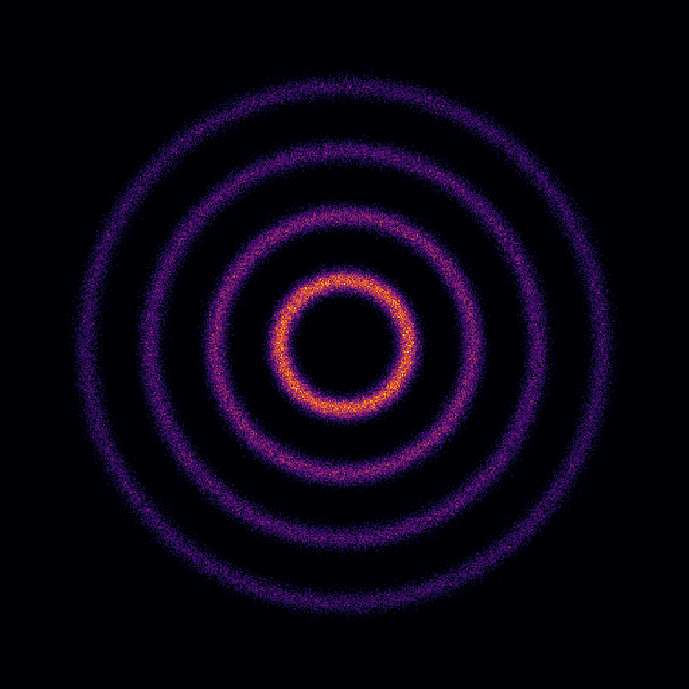
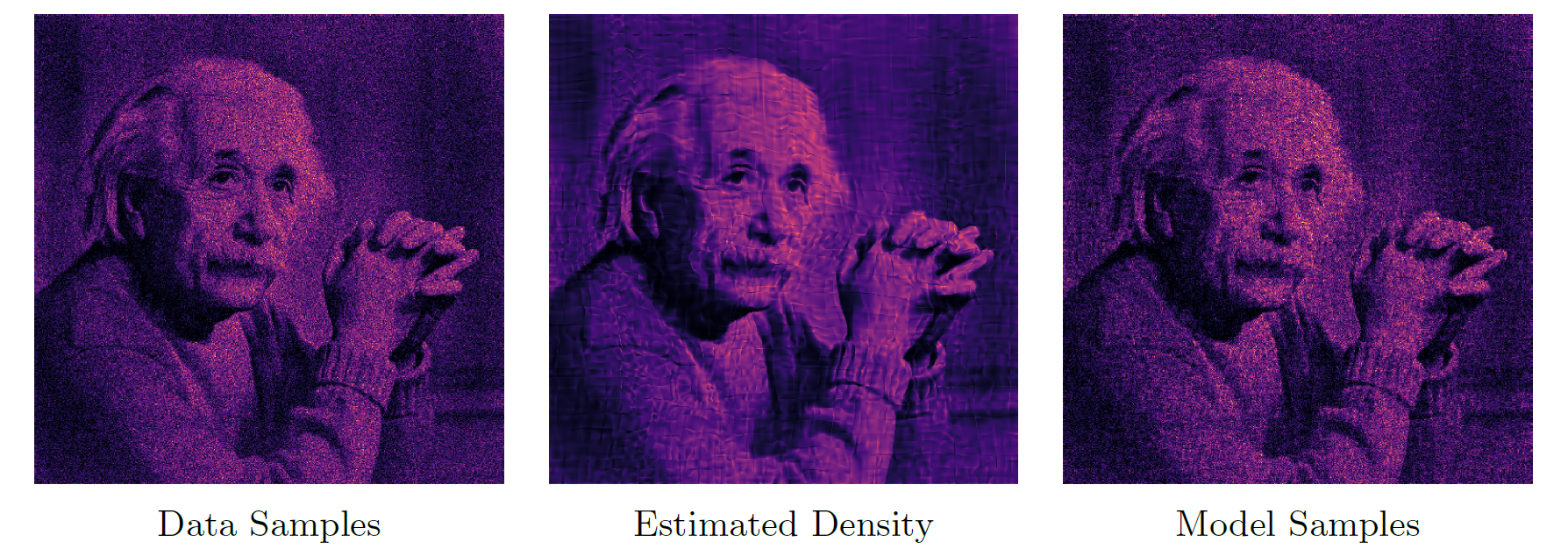
We can even go further and simulate more complicated cases. For example, we can construct 2d data samples based on the intensity of a grayscale image. We can then treat these points as i.i.d. data samples, and try to find their probability density. The figure below shows an example image. As you can see, our method is flexible enough to model such a complicated distribution.

Simulation Results: Image Datasets

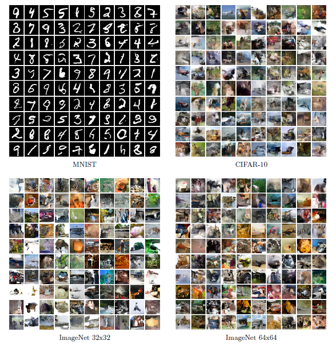
We can use a similar approach for image datasets: assume that they are i.i.d. samples of an unknown probability distribution. With such an assumption, we can use normalizing flows to estimate this density and generate new samples. We also simulate this case for several famous image datasets such as MNIST, CIFAR-10, and ImageNet. Below you can see samples of the flow-based model trained on these datasets.

Concluding Remarks

In this blog post, I provided a brief introduction to normalizing flows. After reviewing flow-based models, we went over the coupling layer transformations. Then, we showed how one can construct a flow-based model using linear rational splines. Finally, we showed a few use-cases of flow-based modeling in synthetic and real-world data. More details can be found in our AISTATS paper. Also, our implementation is available at this repository. Should you have any question, please do not hesitate to contact me.