
AdvFlow: Black-box Adversarial Attacks using Normalizing Flows
Published:
In this blog post, we give an overview of our recent work entitled “AdvFlow: Inconspicuous Black-box Adversarial Attacks using Normalizing Flows.” This work has been accepted to the 34th Conference on Neural Information Processing Systems (NeurIPS 2020). You can find the camera-ready version of the paper here. Also, our implementation is available at this repository.
We begin with a brief introduction to adversarial attacks. Then, we give an overview of search gradients from Natural Evolution Strategies (NES). Afterward, we present AdvFlow that is a combination of normalizing flows with NES for black-box adversarial example generation. Finally, we go over some of the simulation results. Note that some basic familiarity with normalizing flows is assumed in this blog post. We have already written a blog post on normalizing flows that you can find here. So, let’s get started!
Adversarial Attacks
Deep neural networks (DNN) have revolutionized machine learning during the past decade. Today, they are used in various tasks, including speech-to-text translation, object detection, and image segmentation. Despite their huge success, many aspects of their behavior are yet to be fully understood. A particular failure of DNNs that you may have heard of is their adversarial vulnerability.
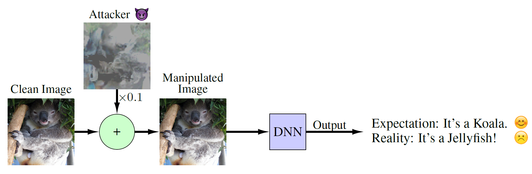
It is shown that DNNs are susceptible to tiny but carefully designed changes in their input. For example, we may have a trained DNN classifier to discriminate different images for us. We expect that for all samples of the same class we get the same output by the classifier. Instead, an input image can be manipulated in a way that while it looks like the original one, the DNN classifier assigns an entirely different label to it. This issue is fundamental and needs to be addressed somehow; otherwise, we may get unwanted behavior from our models in the real-world.
There are numerous ways one can construct such inputs, known as adversarial examples. Here, we assume that image classifiers are the ones that we are going to attack. So, let’s consider a DNN classifier \({\mathcal{C}(\cdot): \mathcal{X}^{d} \rightarrow \mathcal{P}^{k}}\), where \(\mathcal{X}^{d}\) is the set of input images, and \(\mathcal{P}^{k}\) are \(k\)-dimensional probability vectors. When the true class label of an image \(\mathbf{x}\) is \(y\), we expect that the \(y\)-th element of the DNN output \(\mathbf{p}=\mathcal{C}(\mathbf{x})\) would be the maximum one. This way, we can say that the classifier has assigned the correct label to the input image.
As a first step, we need a criterion to define what we exactly mean when we say “a similar image to the true one.” The easiest way of writing down this criterion is to consider all images whose \(\ell_p\) distance to the original image is less than \(\epsilon\). In particular, let \(\mathbf{x}\) denote the original, clean image. Then, we can define the set of similar images to \(\mathbf{x}\) using
\[\label{eq:set}\nonumber \mathcal{S}(\mathbf{x}) = \left\{\mathbf{x}' \in \mathcal{X}^{d}~\big\rvert~\lVert{\mathbf{x}' - \mathbf{x}}\rVert_{p}\leq \epsilon \right\},\]for an appropriate choice of \(\epsilon\).
The next step is to find an image \(\mathbf{x}'\) in the set \(\mathcal{S}(\mathbf{x})\) such that the classifier assigns a wrong label to it. Since we know that the set \(\mathcal{S}(\mathbf{x})\) only contains similar images to the original one \(\mathbf{x}\), we expect our DNN classifier to always output the same correct label. So, when it fails to do so, we can say that we have found an adversarial image. Mathematically, assume that we have a clean image \(\mathbf{x}\) that belongs to the class \(y\). In this case, we expect that the \(y\)-th element of the classifier output would be greater than the rest. In our notation, it translates as
\[\label{eq:corr}\nonumber \forall {c \neq y} ~~~~~~ {\mathcal{C}(\mathbf{x})_{y} > \mathcal{C}(\mathbf{x})_{c}}.\]Now, let’s consider an image \(\mathbf{x}'\) from the set \(\mathcal{S}(\mathbf{x})\). For this image to be adversarial, we need to have \({\mathcal{C}(\mathbf{x}')_{y} \leq \max_{c \neq y} \mathcal{C}(\mathbf{x}')_{c}}\) (why?). This means that while our image \(\mathbf{x}'\) is similar to the true one, the classifier assigns a wrong label to it. Carlini & Wagner rewrite this objective as
\[\label{eq:CW_loss}\nonumber \mathcal{L}(\mathbf{x}')=\max\big\{0, \log \mathcal{C}(\mathbf{x}')_{y} - \max_{c \neq y} \log \mathcal{C}(\mathbf{x}')_{c}\big\}.\]It can be shown that \({\mathcal{L}(\mathbf{x}') \geq 0}\). The minimum occurs whenever \(\mathcal{L}(\mathbf{x}')\) becomes zero. In this case, we are guaranteed to have \({\mathcal{C}(\mathbf{x}')_{y} \leq \max_{c \neq y} \mathcal{C}(\mathbf{x}')_{c}}\) (why?), which is our original objective. Writing the objective this way makes it bounded below, and hence, suitable for numerical minimization.
Finally, we are ready to put all the ingredients together. Remember that we were looking to find similar images to the clean one (or \(\mathbf{x}' \in \mathcal{S}(\mathbf{x})\)) such that the classifier assigns the wrong label to it (or \({\mathcal{C}(\mathbf{x}')_{y} \leq \max_{c \neq y} \mathcal{C}(\mathbf{x}')_{c}}\)). We can write this as the following minimization problem:
\[\label{eq:adv_example} \DeclareMathOperator*{\argmin}{arg\,min} {\mathbf{x}}_{adv}=\argmin_{\mathbf{x}' \in \mathcal{S}(\mathbf{x})} \mathcal{L}(\mathbf{x}').\]If we can find a minimizer to our objective function, we say that we have successfully attacked a DNN classifier.
Black-box vs. White-box Attacks
Now that we have seen what is an adversarial example and how to construct one, let’s go over their categorization. As we saw in Eq. (1), finding an adversarial example is equivalent to solving an optimization problem involving the classifier. Based on the amount of information that we assume to have while attacking a DNN classifier, we can broadly categorize current methods into two: white-box and black-box. In white-box attacks, we assume that we know everything about the target classifier, from its internal architecture to its weights. This way, we can utilize our knowledge about the classifier to take its gradient and minimize Eq. (1). Black-box attacks, however, assume that we do not know anything about the internal structure of the target classifier. We can only query the classifier and see the output. Also, sometimes we have a certain threshold for the number of times that we can query the classifier. Thus, we have to work harder to come up with adversarial examples in this case. In this paper, we design black-box adversarial attacks as they seem to be more realistic.
This concludes our short introduction to adversarial attacks. For a more thorough review, please do check out this amazing NeurIPS tutorial by Madry & Kolter.
Natural Evolution Strategies (NES)
In the previous section, we saw how one can generate an adversarial image by optimizing Eq. (1). Also, we said that we are looking for a way to solve this optimization problem in the black-box setting, meaning that we can only work with the input-output pairs.
This is a well-studied problem in the field of optimization, and there are various ways of solving such problems. A famous approach is the idea of search gradients from Natural Evolution Strategies (NES). Instead of optimizing \(\mathcal{L}(\mathbf{x}')\) directly, NES defines a parametric probability distribution over the set of inputs \(\mathbf{x}'\), and then tries to optimize the expectation of \(\mathcal{L}(\mathbf{x}')\) over this parametric distribution. The parameters of this distribution can then be adjusted so that we get the minimum value on average. As we will see, this procedure does not require taking the gradients of the objective. This property makes NES the perfect candidate for our purposes.
In particular, assume that \({p(\mathbf{x'}\mid\boldsymbol{\psi})}\) denotes the search distribution with parameters \({\boldsymbol{\psi}}\). NES replaces the objective of Eq. (1) with
\[\label{eq:nes} J(\boldsymbol{\psi})=\mathbb{E}_{p(\mathbf{x'}\mid\boldsymbol{\psi})}\left[\mathcal{L}(\mathbf{x}')\right].\]In other words, instead of trying to minimize \(\mathcal{L}(\mathbf{x}')\) directly, we fit a parametric distribution to the set of possible solutions. We do this by minimizing the expectation of our original loss. This means that we expect the distribution \(p(\mathbf{x'}\mid\boldsymbol{\psi})\) to generate samples that on average minimize our loss \(\mathcal{L}(\mathbf{x}')\).
Numerical minimization of \(J(\boldsymbol{\psi})\) requires computing its gradient with respect to \(\boldsymbol{\psi}\). To this end, we can exploit the “log-likelihood trick”:
\[\begin{aligned}\label{eq:ap:LLtrick}\nonumber \nabla_{\boldsymbol{\psi}}J(\boldsymbol{\psi}) &\stackrel{(1)}{=} \nabla_{\boldsymbol{\psi}}\mathbb{E}_{p(\mathbf{x'}\mid\boldsymbol{\psi})}\left[\mathcal{L}(\mathbf{x}')\right]\\\nonumber &\stackrel{(2)}{=} \nabla_{\boldsymbol{\psi}} \int \mathcal{L}(\mathbf{x}') p(\mathbf{x'}\mid\boldsymbol{\psi})\mathrm{d}\mathbf{x}'\\\nonumber &\stackrel{(3)}{=} \int \mathcal{L}(\mathbf{x}') \nabla_{\boldsymbol{\psi}}p(\mathbf{x'}\mid\boldsymbol{\psi})\mathrm{d}\mathbf{x}'\\\nonumber &\stackrel{(4)}{=} \int \mathcal{L}(\mathbf{x}') \frac{\nabla_{\boldsymbol{\psi}}p(\mathbf{x'}\mid\boldsymbol{\psi})}{p(\mathbf{x'}\mid\boldsymbol{\psi})}p(\mathbf{x'}\mid\boldsymbol{\psi})\mathrm{d}\mathbf{x}'\\\nonumber &\stackrel{(5)}{=} \int \mathcal{L}(\mathbf{x}') \nabla_{\boldsymbol{\psi}}\log\big(p(\mathbf{x'}\mid\boldsymbol{\psi})\big) p(\mathbf{x'}\mid\boldsymbol{\psi})\mathrm{d}\mathbf{x}'\\ &\stackrel{(6)}{=} \mathbb{E}_{p(\mathbf{x'}\mid\boldsymbol{\psi})}\left[\mathcal{L}(\mathbf{x}') \nabla_{\boldsymbol{\psi}}\log\big(p(\mathbf{x'}\mid\boldsymbol{\psi})\big)\right]. \end{aligned}\]Here, (1) is the definition of \(J(\boldsymbol{\psi})\), (2) is the definition of expectation, (3) is because we can replace the integration and differentiation order, (4) is a factorization, (5) is by the definition of the \(\log(\cdot)\) gradient, and (6) is again the definition of the expectation. As you see, the gradient of \(J(\boldsymbol{\psi})\) with respect to \(\boldsymbol{\psi}\) only involves querying the objective/classifier.
Now, we can minimize \(J(\boldsymbol{\psi})\) using gradient descent. We first initialize \(\boldsymbol{\psi}\) randomly, and then update it by computing \(\boldsymbol{\psi} \leftarrow \boldsymbol{\psi} - \alpha \nabla_{\boldsymbol{\psi}}J(\boldsymbol{\psi})\) iteratively. Here, \(\alpha\) is the learning rate, and \(\nabla_{\boldsymbol{\psi}}J(\boldsymbol{\psi})=\mathbb{E}_{p(\mathbf{x'}\mid\boldsymbol{\psi})}\left[\mathcal{L}(\mathbf{x}') \nabla_{\boldsymbol{\psi}}\log\big(p(\mathbf{x'}\mid\boldsymbol{\psi})\big)\right]\).
AdvFlow
We are finally ready to present AdvFlows. As we saw earlier, we should define an appropriate distribution \({p(\mathbf{x'}\mid\boldsymbol{\psi})}\) over \(\mathbf{x'}\) to use NES. To this end, we propose to exploit the power of normalizing flows in modeling probability distributions.
As we have already seen in this blog post, normalizing flows model the data distribution via transforming a universal base density (such as standard normal) to the data distribution. To do this, they use stacked layers of invertible neural networks (INN). Specifically, let \(\mathbf{X} \sim p(\mathbf{x})\) denote the data distribution. We can model the data as an appropriately trained INN \(\mathbf{f}(\cdot)\) applied to a standard normal \(\mathbf{Z} \sim p(\mathbf{z})=\mathcal{N}(\mathbf{z}\mid\mathbf{0}, I)\) random vector. This is where the change of variables formula comes into play, helping us to write the distribution of \(\mathbf{X}=\mathbf{f}(\mathbf{Z})\) as
\[\label{eq:change_of_variable}\nonumber p(\mathbf{x}) = p(\mathbf{z})\left|\mathrm{det}\Big(\dfrac{\partial \mathbf{f}}{\partial \mathbf{z}}\Big)\right|^{-1}.\]Here, we are looking to model the distribution of the adversarial examples \(\mathbf{x}' \in \mathcal{S}(\mathbf{x})\). We propose to exploit normalizing flows for this matter. To this end, we first train a flow-based model \(\mathbf{f}(\cdot)\) on the clean data distribution. Since the adversaries look like the clean image, we speculate that their distribution is also following the clean data distribution closely. So, instead of changing the distribution entirely, we only change its base distribution from \(\mathcal{N}(\mathbf{z}\mid\mathbf{0}, I)\) to \(\mathcal{N}(\mathbf{z}\mid\boldsymbol{\mu}, \sigma^2 I)\). Here, \(\boldsymbol{\mu}\) and \(\sigma\) are the NES parameter set \(\boldsymbol{\psi}\), and we treat the flow-based model \(\mathbf{f}(\cdot)\) as a fixed transformation. In other words, we write:
\[\label{eq:advflow_dist} \mathbf{x}'=\mathrm{proj}_{\mathcal{S}}\big(\mathbf{f}(\mathbf{z})\big),\qquad\mathbf{z}\sim\mathcal{N}(\mathbf{z}\mid\boldsymbol{\mu}, \sigma^2 I)\]where \(\mathrm{proj}_{\mathcal{S}}(\cdot)\) projects the adversaries to the set \(\mathcal{S}(\mathbf{x})\). Now, we can re-write Eq. (2) for our choice of distribution as:
\[\begin{aligned}\label{eq:advflow_cost} J(\boldsymbol{\psi}) &\stackrel{(1)}{=} J(\boldsymbol{\mu}, \sigma) \nonumber\\ &\stackrel{(2)}{=} \mathbb{E}_{p(\mathbf{x'}\mid\boldsymbol{\mu}, \sigma)}\left[\mathcal{L}(\mathbf{x}')\right] \nonumber\\ &\stackrel{(3)}{=} \mathbb{E}_{\mathcal{N}(\mathbf{z}\mid\boldsymbol{\mu}, \sigma^2 I)}\left[\mathcal{L}\bigg(\mathrm{proj}_{\mathcal{S}}\big(\mathbf{f}(\mathbf{z})\big)\bigg)\right]. \end{aligned}\]In this derivation, (1) is because we defined \(\boldsymbol{\psi}=\{\boldsymbol{\mu}, \sigma\}\), (2) is the definition of our surrogate objective, and (3) is due to the rule of the lazy statistician. Next, we should compute the gradient of \(J(\boldsymbol{\mu}, \sigma)\) with respect to \(\boldsymbol{\psi}=\{\boldsymbol{\mu}, \sigma\}\). To decrease the computational burden, we set \(\sigma\) by hyper-parameter tuning, and only optimize \(\boldsymbol{\mu}\). The gradient \(\nabla_{\boldsymbol{\mu}}J(\boldsymbol{\mu}, \sigma)\) can be computed using Eq. (3) as
\[\label{eq:jac_advflow} \nabla_{\boldsymbol{\mu}}J(\boldsymbol{\mu}, \sigma) = \mathbb{E}_{\mathcal{N}(\mathbf{z}\mid\boldsymbol{\mu}, \sigma^2 I)}\left[\mathcal{L}\bigg(\mathrm{proj}_{\mathcal{S}}\big(\mathbf{f}(\mathbf{z})\big)\bigg) \nabla_{\boldsymbol{\mu}}\log \mathcal{N}(\mathbf{z}\mid\boldsymbol{\mu}, \sigma^2 I)\right].\]A nice property of this equation is that \(\nabla_{\boldsymbol{\mu}}\log \mathcal{N}(\mathbf{z}\mid\boldsymbol{\mu}, \sigma^2 I)\) can be computed in closed-form. Hence, in each iteration of AdvFlow, we first generate some samples \(\mathbf{z}_i\) from the distribution \(\mathcal{N}(\mathbf{z}\mid\boldsymbol{\mu}, \sigma^2 I)\). We then evaluate \(\mathcal{L}\bigg(\mathrm{proj}_{\mathcal{S}}\big(\mathbf{f}(\mathbf{z}_i)\big)\bigg)\) and \(\nabla_{\boldsymbol{\mu}}\log \mathcal{N}(\mathbf{z}_i\mid\boldsymbol{\mu}, \sigma^2 I)\) for these samples. Then, \(\nabla_{\boldsymbol{\mu}}J(\boldsymbol{\mu}, \sigma)\) is approximated by forming the average of \(\mathcal{L}\bigg(\mathrm{proj}_{\mathcal{S}}\big(\mathbf{f}(\mathbf{z}_i)\big)\bigg) \nabla_{\boldsymbol{\mu}}\log \mathcal{N}(\mathbf{z}_i\mid\boldsymbol{\mu}, \sigma^2 I)\) over \(i\), and we can finally use this approximation to update \({\boldsymbol{\mu}}\) by
\[\label{eq:advflow_update} \boldsymbol{\mu} \leftarrow \boldsymbol{\mu} - \alpha \nabla_{\boldsymbol{\mu}}J(\boldsymbol{\mu}, \sigma).\]To help the algorithm converge faster, we first map the clean image \(\mathbf{x}\) to its base distribution representation by \(\mathbf{z}=\mathbf{f}^{-1}(\mathbf{x})\). We then add a small additive vector \({\boldsymbol{\delta}_z}=\boldsymbol{\mu} + \sigma \boldsymbol{\epsilon}\) (where \(\boldsymbol{\epsilon}\sim\mathcal{N}(\boldsymbol{\epsilon}\mid\mathbf{0}, I)\)) to \(\mathbf{z}\) to be our adversarial example representation in the base distribution space. This step makes total sense: as we expect our adversarial image to be close to the clean image, their latent representations are also going to be close. This conclusion is due to the differentiability and also invertibility of the normalizing flows.
This concludes AdvFlows for black-box adversarial example generation. You can see a step-by-step procedure in the GIF below.
AdvFlow Interpretations
There are two beautiful interpretations of AdvFlows. First, we can think of AdvFlows as a search over the base distribution of flow-based models. We map the clean image to the latent space and then try to search in the neighborhood of our image in the base distribution space for an adversarial image. Since we have pre-trained the flow-based model, the adversarial examples are going to be like the clean data, with the perturbations taking the structure of the data.
Secondly, and more importantly, we can interpret AdvFlows from a distributional perspective. We first initialize the distribution of adversarial images with that of the clean data. The only difference is that we transform the base distribution by an affine mapping. This tiny change would help us change the clean data distribution into one that generates adversarial examples!
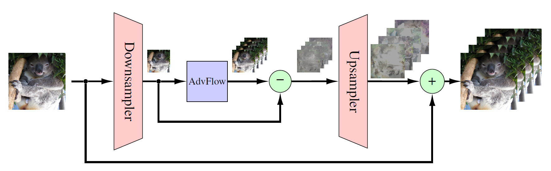
AdvFlow for High-resolution Images
Although flow-based models have seen a lot of advances in recent months, their application to high-resolution image data is still computationally expensive. To deal with this issue, we propose a small adjustment to our original AdvFlow framework so that we can use them for high-resolution data. To this end, we decrease the resolution of the clean image and try to come up with an adversarial image in a low-dimensional space using AdvFlow. Then, we compute the difference between the clean and adversarial images in the low-dimensional space and map the difference to high-dimensions using a bilinear up-sampler. This difference is then added to the clean, high-resolution image to give our adversarial image. The diagram of this adjustment is shown below.
Simulation Results
In this section, we present the most important simulation results. You can find the details as well as more simulation results in our paper.
Fooling Adversarial Example Detectors
One approach to defend DNN classifiers against adversarial attacks is through adversarial example detectors. This way, a detector is trained and put before the classifier. Whenever an input is sent to the classifier, first it has to pass the detector to determine whether it is adversarial or not.
There are various adversarial example detectors. A common assumption among such methods is that the adversarial examples come from a different distribution than the clean data. From this perspective, they suit our purpose of assessing whether AdvFlows generate adversarial examples that follow the clean data distribution or not.
We compare AdvFlows with a similar distributional black-box attack method called \(\mathcal{N}\)Attack. We pre-train the flow-based part of our model using clean training data. As an ablation study, we also take a randomly initialized AdvFlow into account to see the effect of the pre-training.
Table 1 shows the detection rate (in AUROC) and the accuracy of three adversarial example detectors for the black-box adversarial examples generated by AdvFlow and \(\mathcal{N}\)Attack. As seen, the detection of trained AdvFlow attacks is more difficult than \(\mathcal{N}\)Attack. This supports our statement earlier that AdvFlows result in adversarial examples that are closer to the clean data distribution. Also, you see that before training the flow-based model, AdvFlows generate adversarial examples that are easily detectable. This indicates the importance of pre-training the flow-based models on clean data.
Table: Area under the receiver operating characteristic curve (AUROC) and accuracy of detecting adversarial examples generated by NATTACK and AdvFlow (un. for un-trained and tr. for pre-trained NF) using LID, Mahalanobis, and Res-Flow adversarial attack detectors.
| Data | Metric | AUROC(%) | Detection Acc.(%) | ||||
|---|---|---|---|---|---|---|---|
| Method | 𝒩Attack | AdvFlow (un.) | AdvFlow (tr.) | 𝒩Attack | AdvFlow (un.) | AdvFlow (tr.) | |
| CIFAR-10 | LID | 78.69 | 84.39 | 57.59 | 72.12 | 77.11 | 55.74 |
| Mahalanobis | 97.95 | 99.50 | 66.85 | 95.59 | 97.46 | 62.21 | |
| Res-Flow | 97.90 | 99.40 | 67.03 | 94.55 | 97.21 | 62.60 | |
| SVHN | LID | 57.70 | 58.92 | 61.11 | 55.60 | 56.43 | 58.21 |
| Mahalanobis | 73.17 | 74.67 | 64.72 | 68.20 | 69.46 | 60.88 | |
| Res-Flow | 69.70 | 74.86 | 64.68 | 64.53 | 68.41 | 61.13 | |
Fooling Vanilla and Defended Classifiers
As our final simulation result, we see the performance of AdvFlows in contrast to Bandits \& Priors, \(\mathcal{N}\)Attack, and SimBA. For the defended classifiers, we use fast adversarial training. The architecture of our models is the famous ResNet-50. We set the maximum number of queries to 10,000 and try to attack both vanilla and adversarially trained classifiers.
Table 2 shows our simulation results for CIFAR-10, SVHN, and ImageNet datasets. For CIFAR-10 and SVHN we apply AdvFlows directly, while for ImageNet we use the alternative version of AdvFlows. As can be seen, our method improves upon the performance of the baselines in the defended scenarios.
Table: Success rate and the average number of queries in attacking CIFAR-10, SVHN, and ImageNet classifiers. For a fair comparison, we first find the samples where all the attack methods are successful, and then compute the average of queries among these samples. All attacks are with respect to \(\ell_{\infty}\) norm with \(\epsilon=8/255\).
| Data | Architecture | Clean Acc(%) | Success Rate(%) | Average Number of Queries | ||||||
|---|---|---|---|---|---|---|---|---|---|---|
| Bandits | \(\mathcal{N}\)Attack | SimBA | AdvFlow (ours) | Bandits | \(\mathcal{N}\)Attack | SimBA | AdvFlow (ours) | |||
| CIFAR-10 | Van. ResNet | 91.75 | 96.75 | 99.85 | 99.96 | 99.37 | 795.28 | 252.13 | 286.05 | 1051.18 |
| Def. ResNet | 79.09 | 45.20 | 45.19 | 43.57 | 49.08 | 891.54 | 901.44 | 374.58 | 359.21 | |
| SVHN | Van. ResNet | 96.23 | 92.63 | 96.73 | 93.14 | 83.67 | 1338.30 | 487.32 | 250.02 | 1749.48 |
| Def. ResNet | 92.67 | 43.26 | 36.99 | 38.98 | 45.11 | 739.40 | 1255.24 | 286.71 | 436.83 | |
| ImageNet | Van. ResNet | 95.00 | 95.79 | 99.47 | 98.42 | 95.58 | 948.90 | 604.31 | 701.92 | 1501.13 |
| Def. ResNet | 71.50 | 50.77 | 33.99 | 47.55 | 57.20 | 914.58 | 2170.82 | 969.91 | 381.97 | |
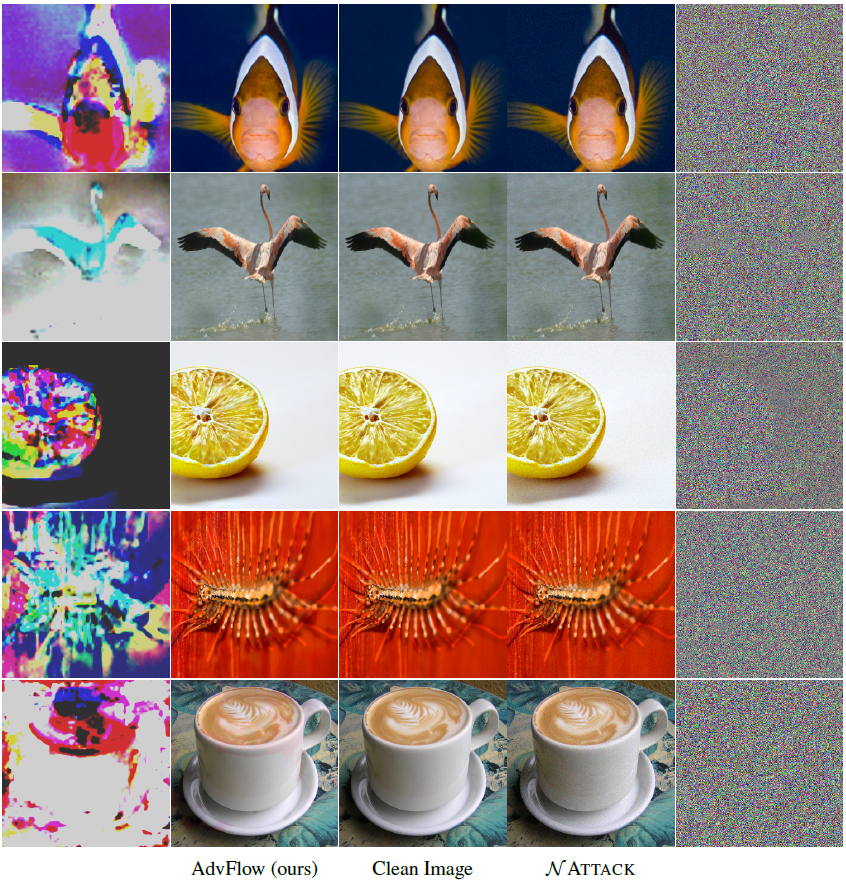
Finally, below you can see adversarial examples generated by AdvFlow and \(\mathcal{N}\)Attack. As you can see, our approach generates perturbations that look like clean data while this is not the case for \(\mathcal{N}\)Attack.
Conclusion
In this short blog post, we covered the general idea of designing black-box adversarial attacks using normalizing flows, resulting in an algorithm we called AdvFlow. The most interesting property of AdvFlows is that they provide a close connection between clean and adversarial data distributions. We saw the effectiveness of the proposed approach in fooling adversarial example detectors that assume adversaries come from a different density than the intact data. For more details, please read the camera ready version of our paper. Also, you can find the PyTorch implementation of AdvFlows at this repository. Should you have any questions, I would be happy to have a chat with you. Take care!