Denoising Diffusion Probabilistic Models
Published:
In this blog post, I will give a brief overview of the diffusion models used in the paper “Denoising Diffusion Probabilistic Models” by Ho et al. The official repository of the paper contains their code in TensorFlow. I also created an unofficial repository written in PyTorch and Pytorch-Lightning that you can find here.
Introduction
Informally, generative modeling is a branch of machine learning that is concerned with finding the hidden process by which a given dataset is generated. In other words, it is assumed that there is an unknown machinery that has generated the data in hand, and our goal is to find this hidden process. Given a wide variety of data out there, this task is particularly challenging when it comes to high-dimensional data such as images with thousands of pixels. Once the generative process is estimated, it can be used in a suite of applications such as data augmentation, compression, etc.
The first step in solving this problem is to make some assumptions about the nature of the generative process by which we believe the data has been created. It is common to assume that the data are realizations of a random variable, and there is a probability density that has generated the data. This way, one can rely on mature fields such as statistics and use their tools developed over the years in estimating the generative processes.
Only making the assumption that our generative process is some form of probability density is not enough. Because there are infinite number of possibilities that we can model our data generation. We further need to specify the family of distributions that we “assume” is behind generating the data. In this regard, the world of plausible models is immense. For example, we might assume that our image dataset is generated by some simple probabilistic model such as Gaussian Mixture Models, or consider more involved density models such as normalizing flows. In this paper, the authors propose using diffusion models as a generative model for high-dimensional image data.
Diffusion Models
Markov Chains
Before jumping into the definition of diffusion models, let’s review Markov chains.
Chains are a natural way to stochastically represent a model’s evolution over time. A random variable is assigned to the model outcome at different observation times, representing various states of the model. The relationship of these states can then be formulated using conditional probability densities.
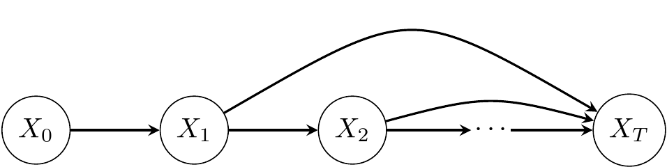
In particular, let’s assume that our model starts at some point \(t=0\) in time. We can assign a random variable \(X_{0} \sim p(x_{0})\) to probabilistically represent the state of our model at this time \(t=0\). Then, based on its value at time \(t=0\), our model evolves and changes its state. Now, if we denote the model state at time \(t=1\) with random variable \(X_{1}\), we can formulate the change of state from \(X_{0}\) to \(X_{1}\) by the conditional probability \(p(x_{1} \mid x_{0})\). In other words, we assumed that our model state at time \(t=1\) is a consequence of its state at time \(t=0\). We can then go on and repeat this procedure for an arbitrary time \(t=T\): representing the current state with random variable \(X_T\), the relationship of the model state at \(t=T\) with its previous states at \(t=T-1,~T-2,~\dots~,~1,~0\) is formulated through \(p(x_{T} \mid x_{T-1},~x_{T-2},~\dots~,~x_{0})\). Having defined these densities, we can compute the joint probability distribution of all model states using the product rule:
\[\begin{aligned}\nonumber p(x_{T},~x_{T-1},~x_{T-2},~\dots~,~x_{0}) &= p(x_{T} \mid x_{T-1},~x_{T-2},~\dots~,~x_{0})~\cdots~p(x_{1} \mid x_{0})~p(x_{0})\\&=p(x_{0}) \prod_{t=1}^{t=T} p(x_{t} \mid x_{<t}). \end{aligned}\]Now, a Markov chain is a simplification of this general rule: each state \(t\) only depends on its previous state \(t-1\), not the whole sequence of states from the beginning. This way, we can simplify our previous equation as:
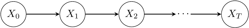
\[\nonumber p(x_{T},~x_{T-1},~x_{T-2},~\dots~,~x_{0}) =p(x_{0}) \prod_{t=1}^{t=T} p(x_{t} \mid x_{t-1}).\]In graphical model representation, we can depict chains as follows.
Using the same notation, Markov chains can be shown as
Diffusion Models
Now that we know Markov chains, defining diffusion models is straightforward. As stated in the introduction, in probabilistic generative modeling we assume that our data \(\mathbf{x}_{0}\) is generated by an unknown density \(p^{*}(\mathbf{x}_{0})\). We model this data generating distribution with some \(p_{\boldsymbol{\theta}}(\mathbf{x}_{0})\), and try to fit our model parameters \(\boldsymbol{\theta}\) to data observations \(\{\mathbf{x}_{0}^{0},~\mathbf{x}_{0}^{1},~\dots,~\mathbf{x}_{0}^{n-1}\}\).
In diffusion models, the data generating process is defined using two Markov chains. These chains are defined over the sequence \(\{\mathbf{x}_{0},~\mathbf{x}_{1},~\dots,~\mathbf{x}_{T}\}\), where \(\mathbf{x}_{0}\) denotes our data vector and the rest are some latent, hidden variables. A latent variable is one that we assume is contributing to the generation of data, but we never get to observe it. Here, the latent variables are going to capture the gradual formation of data from random noise in form of a standard normal distribution \(\mathbf{x}_{T} \sim \mathcal{N}(\mathbf{x}_{T};~\mathbf{0},~\mathbf{I})\).
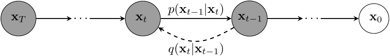
The first Markov chain starts from random noise \(\mathbf{x}_{T}\) and gradually decreases its index until it reaches \(\mathbf{x}_{0}\). As you can see, we are somehow going in the opposite direction of time, and I believe this is why this Markov chain is called the reverse process. The interesting point about diffusion models is that not only the starting point \(\mathbf{x}_{T}\) is defined to be a Gaussian, but all the conditional probability densities that define the chain:
\[\nonumber p_{\boldsymbol{\theta}}(\mathbf{x}_{t-1} \mid \mathbf{x}_{t}) = \mathcal{N}\big(\mathbf{x}_{t-1};~\boldsymbol{\mu}_{\boldsymbol{\theta}}(\mathbf{x}_{t},~t),~\boldsymbol{\Sigma}_{\boldsymbol{\theta}}(\mathbf{x}_{t},~t)\big).\]Here, \(\boldsymbol{\mu}_{\boldsymbol{\theta}}(\mathbf{x}_{t}, t)\) and \(\boldsymbol{\Sigma}_{\boldsymbol{\theta}}(\mathbf{x}_{t},~t)\) denote the mean and covariance of the Gaussian distribution. As seen, they are functions of the condition \(\mathbf{x}_{t}\) and time \(t\). In denoising diffusion probabilistic models, \(\boldsymbol{\mu}_{\boldsymbol{\theta}}(\mathbf{x}_{t},~t)\) is implemented with a type of neural network called U-net, while \(\boldsymbol{\Sigma}_{\boldsymbol{\theta}}(\mathbf{x}_{t},~t)\) is set to time-dependent constants \(\sigma_t^2\mathbf{I}\).
So, now that we have all the conditional probability densities defined, we can write down the joint probability density of random vectors \(\{\mathbf{x}_{0}, \mathbf{x}_{1}, \dots, \mathbf{x}_{T}\}\) as:
\[\nonumber p_{\boldsymbol{\theta}}(\mathbf{x}_{0},~\mathbf{x}_{1},~\dots,~\mathbf{x}_{T}) = p(\mathbf{x}_{T}) \prod_{t=1}^{t=T} p_{\boldsymbol{\theta}}(\mathbf{x}_{t-1} \mid \mathbf{x}_{t}).\]Since the variables \(\{\mathbf{x}_{1},~\mathbf{x}_{2},~\dots,~\mathbf{x}_{T}\}\) are latent, we should marginalize the density \(p(\mathbf{x}_{0},~\mathbf{x}_{1},~\dots,~\mathbf{x}_{T})\) over them to obtain the data density itself
\[\nonumber p_{\boldsymbol{\theta}}(\mathbf{x}_{0}) = \int p_{\boldsymbol{\theta}}(\mathbf{x}_{0},~\mathbf{x}_{1},~\dots,~\mathbf{x}_{T})~\mathrm{d}\mathbf{x}_{1} \cdots~\mathrm{d}\mathbf{x}_{T}.\]To optimize our model parameters we need to compute the aforementioned density for data samples and maximize the parameters log-likelihood. However, computing this integral for arbitrary \(\boldsymbol{\mu}_{\boldsymbol{\theta}}(\mathbf{x}_{t},~t)\) and \(\boldsymbol{\Sigma}_{\boldsymbol{\theta}}(\mathbf{x}_{t},~t)\) is intractable. A common method to deal with this type of situations is estimating the posterior of the model \(p_{\boldsymbol{\theta}}(\mathbf{x}_{1},~\dots,~\mathbf{x}_{T} \mid \mathbf{x}_{0})\) with some density \(q(\mathbf{x}_{1},~\dots,~\mathbf{x}_{T} \mid \mathbf{x}_{0})\) and then maximizing a lower bound of the true log-likelihood knows as the Evidence Lower Bound (ELBO) (the ELBO is for another post! :D). Here the second Markov chain in diffusion models comes into play, where the posterior \(q(\mathbf{x}_{1},~\dots,~\mathbf{x}_{T} \mid \mathbf{x}_{0})\) is defined as
\[\nonumber q(\mathbf{x}_{1},~\dots~,~\mathbf{x}_{T}~\mid~\mathbf{x}_{0}) = \prod_{t=1}^{t=T} q(\mathbf{x}_{t} \mid \mathbf{x}_{t-1}),\]where \(q(\mathbf{x}_{t} \mid \mathbf{x}_{t-1}) = \mathcal{N}(\mathbf{x}_{t}; \sqrt{1-\beta_{t}}\mathbf{x}_{t-1},~\beta_{t}\mathbf{I})\). Since we want to gradually make our data noisy, it makes sense to gradually increase the posterior variance \(\beta_{t}\) over time. Using this posterior, the ELBO can be written as
\[\begin{aligned}\nonumber \mathbb{E}\left[\log p_{\theta}\left(\mathbf{x}_{0}\right)\right] &\geq \mathbb{E}_{q}\left[\log \frac{p_{\theta}\left(\mathbf{x}_{0},~\mathbf{x}_{1},~\dots,~\mathbf{x}_{T}\right)}{q\left(\mathbf{x}_{1},~\mathbf{x}_{2},~\dots,~\mathbf{x}_{T} \mid \mathbf{x}_{0}\right)}\right]\\ &=\mathbb{E}_{q}\left[\log p\left(\mathbf{x}_{T}\right)+\sum_{t = 1}^{T} \log \frac{p_{\theta}\left(\mathbf{x}_{t-1} \mid \mathbf{x}_{t}\right)}{q\left(\mathbf{x}_{t} \mid \mathbf{x}_{t-1}\right)}\right]. \end{aligned}\]Since in \(q(\mathbf{x}_{1},~\dots,~\mathbf{x}_{T} \mid \mathbf{x}_{0})\) we are going in the direct direction of time, this chain is called the forward process. Below you can see a graphical representation of diffusion models.
That concludes diffusion models. Ho et al. use this model and simplify its objective function to get a wighted version of the original ELBO above. The details of this simplification can be read in their paper.